Idea and Implementation / Bayes Theorem and Gaussian Naive Bayes
Bayes Theroem
Any naive bayes approach including Gaussian Naive Bayes depends on the Bayes Theorem. Bayes theorem gives us the probability of an event, given that we have some extra knowledge about that event.
This is the mathmatical definition of the theorem. Here, and are events and
- a conditional probability. It is read as the likelyhood of event A occuring given that event B is true. In an experiment this is our objective variable.
- is prior probability. We are supposed to observe the value of this in our experiment.
- is the conditional probability of B happening given A true.
There is a rather intuitive explanation behind this legendary theroy.
Smoke and Fire Experiment
Our hypothesis is that there will be fire if there is smoke. So, we are asking for . To answer that we’ll start with an experiment sample.

When we collect data about Fire and No Fire events, the area of the white square represents the total sample space.

And we see that we area on the left is Fire and on the right is No Fire samples.
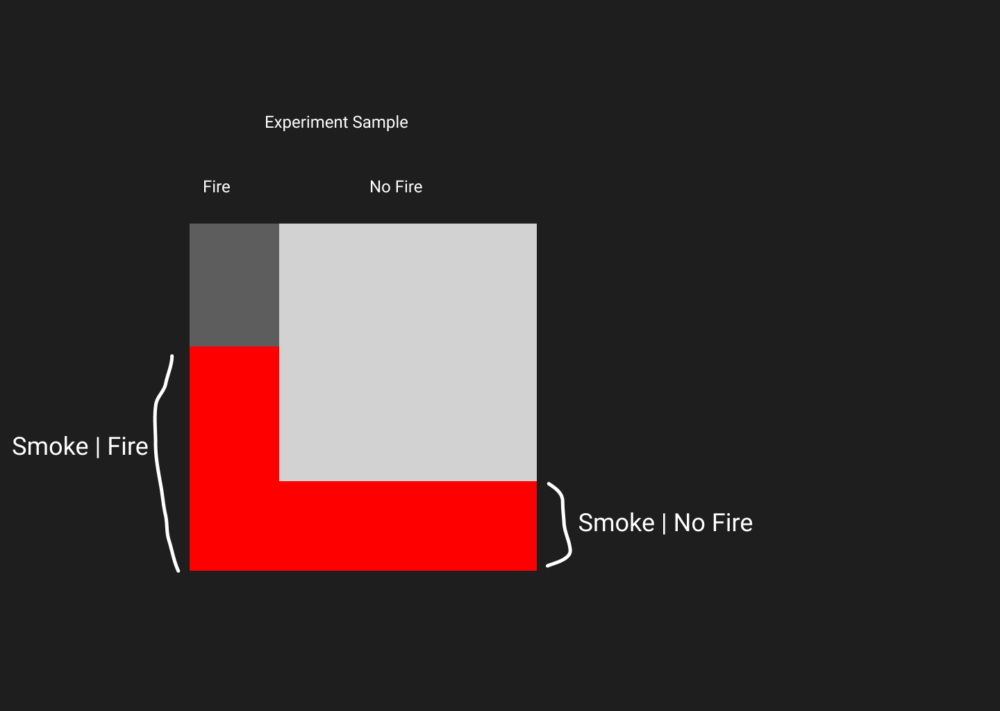
Now let’s observe in which samples smoke was seen in a fire, and in which sample smoke was seen even though there were no fire. Note that, smoke seen in a fire can be written as and not seen in a fire can be written as . Red areas represents smoke was seen. These red areas that I have drawn is based on gut feeling. Smoke is common when there’s a fire, so red area is bigger compared to the red area when there is no fire. Now, as we know probability of something happening is effectively the ratio of that thing against all other thing. Hence, is equals to red area inside fire divided by total red are in experiment.
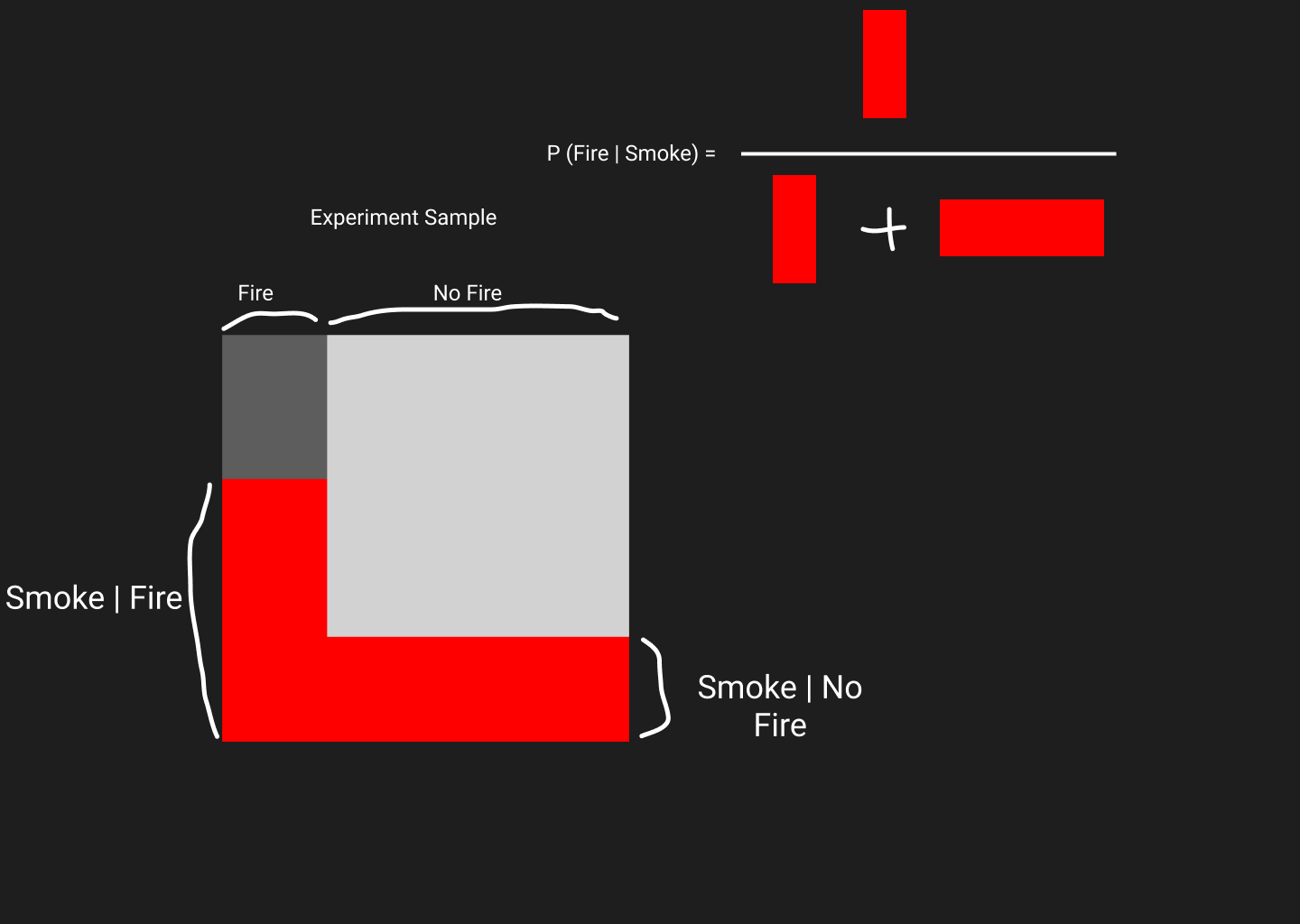
But how the red areas can be calculated mathematically? Well, area is the product of height and width. In our experiment, height is the and width is . Similarly the red area in No Fire can be calculated.
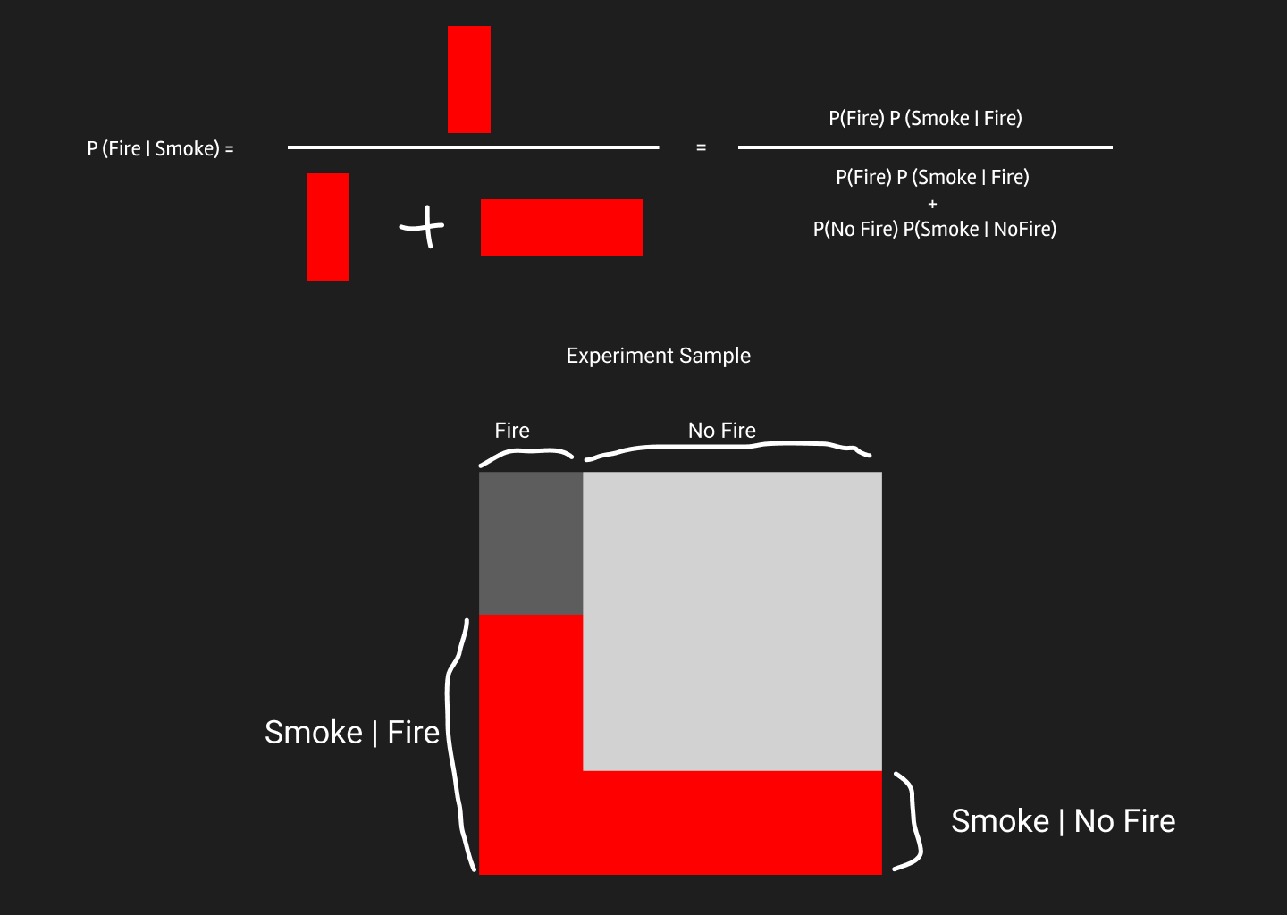
So, we finally get this equation on top.
Note: This is just a geometrical explanation of Bayes Theorem. Gaussian Naive Bayes and other naive bayes algorithms differentiate themselves from this by how they calculate .
Gaussian Naive Bayes
This algorithm assumes likelyhoods of features are of gaussian distribution.
Implementation
We need to calculate priors,, mean and standard deviation, of all features for each available classes in y. Then a function to crunch the above formula of
import math

import numpy as np # linear algebra
import pandas as pd # data processing, CSV file I/O (e.g. pd.read_csv)

from sklearn.datasets import load_iris
from sklearn.model_selection import train_test_split
from sklearn.naive_bayes import GaussianNB
from sklearn.metrics import accuracy_score
class GaussNB:

    def __init__(self):
        """
        No params are needed for basic functionality.
        """
        pass

    def _mean(self,X): # CHECKED
        """
        Returns class probability for each
        """
        mu = dict()
        for i in self.classes_:
            idx = np.argwhere(self.y == i).flatten()
            mean = []
            for j in range(self.n_feats):
                mean.append(np.mean( X[idx,j] ))
            mu[i] = mean
        return mu

    def _stddev(self,X): # CHECKED
        sigma = dict()
        for i in self.classes_:
            idx = np.argwhere(self.y==i).flatten()
            stddev = []
            for j in range(self.n_feats):
                stddev.append( np.std(X[idx,j]) )
            sigma[i] = stddev
        return sigma

    def _prior(self): # CHECKED
        """Prior probability, P(y) for each y
        """
        P = {}
        for i in self.classes_:
            count = np.argwhere(self.y==i).flatten().shape[0]
            probability = count / self.y.shape[0]
            P[i] = probability
        return P

    def _normal(self,x,mean,stddev): # CHECKED
        """
        Gaussian Normal Distribution
        $P(x_i \mid y) = \frac{1}{\sqrt{2\pi\sigma^2_y}} \exp\left(-\frac{(x_i - \mu_y)^2}{2\sigma^2_y}\right)$
        """

        multiplier = (1/ float(np.sqrt(2 * np.pi * stddev**2)))
        exp = np.exp(-((x - mean)**2 / float(2 * stddev**2)))
        return multiplier * exp


    def P_E_H(self,x,h):
        """
        Uses Normal Distribution to get, P(E|H) = P(E1|H) * P(E2|H) .. * P(En|H)

        params
        ------
        X: 1dim array.
            E in P(E|H)
        H: class in y
        """
        pdfs = []

        for i in range(self.n_feats):
            mu = self.means_[h][i]
            sigma = self.stddevs_[h][i]
            pdfs.append( self._normal(x[i],mu,sigma) )

        p_e_h = np.prod(pdfs)
        return p_e_h


    def fit(self, X, y):
        self.n_samples, self.n_feats = X.shape
        self.n_classes = np.unique(y).shape[0]
        self.classes_ = np.unique(y)
        self.y = y

        self.means_ = self._mean(X) # dict of list {class:feats}
        self.stddevs_ = self._stddev(X) # dict of list {class:feat}
        self.priors_ = self._prior() # dict of priors

    def predict(self,X):
        samples, feats = X.shape
        if samples!=self.n_samples or feats!=self.n_feats:
            raise DimensionError("No dimension match with training data!")

        result = []
        for i in range(samples):
            distinct_likelyhoods = []
            for h in self.classes_:
                tmp = self.P_E_H(X[i],h)
                distinct_likelyhoods.append( tmp * self.priors_[h])
            marginal = np.sum(distinct_likelyhoods)
            tmp = 0
            probas = []
            for h in self.classes_:
                numerator = self.priors_[h] * distinct_likelyhoods[tmp]
                denominator = marginal
                probas.append( numerator / denominator )
                tmp+=1
            # predicting maximum
            idx = np.argmax(probas)
            result.append(self.classes_[idx])
        return result
X, y = load_iris(return_X_y=True)
X_train, X_test, y_train, y_test = train_test_split(X, y, test_size=0.5, random_state=0)
gnb = GaussianNB()
sk_pred = gnb.fit(X_train, y_train).predict(X_test)
print("Sci-kit Learn: ",accuracy_score(y_test,sk_pred))

nb = GaussNB()
nb.fit(X_train,y_train)
me_pred = nb.predict(X_test)
print("Custom GaussNB: ",accuracy_score(y_test,me_pred))
Comments